# Chargement des librairies
library(tidyverse)
library(sf)
library(tmap)
library(plotly)
library(gtsummary)
library(GGally)
library(GWmodel)
library(spdep)Régression géographiquement pondérée
Avant-propos
Les données de transcations immobilières utilisées ici (données DVF, pour Demandes de Valeurs Foncières), disponibles sous licence ouverte depuis 2019, sont réputées globalement fiables et exhaustives, mais nécessitent néanmoins des précautions d’utilisation (voir une description de leur qualité ici : https://www.groupe-dvf.fr/vademecum-fiche-n3-precautions-techniques-et-qualite-des-donnees-dvf/). La base utilisée ci-dessous a été retravaillée par etalab, un département de la direction interministérielle du numérique.
L’utilisation de ce jeu de données est ici réalisé dans un but exclusivement pédagogique, et non académique. Par conséquent, la qualité de la donnée n’a pas été re-vérifiée de façon approfondie, et il convient de rester prudent quant aux inférences issues de ces analyses.
1 Objectif de ce support
L’objectif est de mettre en pratique, dans R, certains des concepts et méthodes fréquemment employés en analyse spatiale, avec un focus ici sur l’hétérogénéité spatiale et la régression géographiquement pondérée (GWR). Ce support avait été présenté à l’école d’été SIGR en juillet 2021 (organisée par l’UMS RIATE) et est également disponible en tant que fiche Rzine ici : https://sigr2021.github.io/gwr/
L’hétérogénéité spatiale fait partie de deux principaux concepts de l’analyse spatiale (aux côtés de la dépendance spatiale). Cette hétérogénéité est ubiquiste et systématique, et a pour conséquence qu’aucun lieu sur terre ne saurait être représentatif de tous les autres. Elle a un rôle fondamental dans les analyses géographiques, en particulier quantitatives (elle est indissociable des problèmes de représentativité spatiale, de résolution et d’échelle d’analyse).
D’un point de vue statistique, la traduction de l’hétérogénéité spatiale est la non-stationnarité spatiale. Celle-ci désigne l’instabilité, dans l’espace, des moyennes, des variances et des covariances. La non-stationnarité spatiale des covariances fait référence à l’hétérogénéité spatiale des relations statistiques. C’est cet élément qui fait l’objet de la démonstration ci-dessous.
L’hétérogénéité spatiale des relations statistiques est très fréquente, dans de nombreux domaines (écologie, santé, économie, etc.), et son ignorance peut induire des erreurs d’interprétation importantes et des conséquences économiques et sanitaires (par exemple) non négligeables.
Dans le domaine des marchés immobiliers, cette hétérogénéité spatiale des relations est habituelle. Par exemple, on sait que l’effet marginal d’1 m\(^2\) supplémentaire sur le prix de vente est variable selon la localisation (typiquement plus élevé en zone dense, dans les centres-villes). Cela a des conséquences sur l’estimation des marchés, mais aussi en modélisation hédonique, sur l’estimation de la valeur de différentes caractéristiques sur la base de ces relations.
Cela a poussé des auteurs à segmenter les marchés immobiliers en sous-marchés homogènes, au sein desquels les déterminants du prix seraient stationnaires (voir par exemple Goodman et Thibodeau (1998) ou Helbich et al. (2013)). La question est de savoir comment délimiter ces sous-marchés de façon pertinente.
La méthode proposée dans le cadre de ce cours, la GWR, est une méthode de régression locale qui permet précisément d’explorer la non-stationarité spatiale à travers des cartes de relations (Fotheringham et al., 2003), et de servir alors de base pour une régionalisation. Nous allons préciser la façon dont ce type de modèle est calibré, estimé et interprété.
2 Import et préparation de la base
La base est disponible et décrite ici : https://www.data.gouv.fr/fr/datasets/demandes-de-valeurs-foncieres-geolocalisees/
On importe directement le csv dans R (pour le département 17) :
# Import de la base brute
data <- read_csv("https://files.data.gouv.fr/geo-dvf/latest/csv/2020/departements/17.csv.gz")
# Vérifier que l'import est correct
head(data)# A tibble: 6 × 40
id_mutation date_mutation numero_disposition nature_mutation valeur_fonciere
<chr> <date> <chr> <chr> <dbl>
1 2020-114158 2020-07-01 000001 Vente 576000
2 2020-114159 2020-07-01 000002 Vente 200000
3 2020-114160 2020-07-01 000001 Vente 540800
4 2020-114160 2020-07-01 000001 Vente 540800
5 2020-114161 2020-07-01 000001 Vente 162000
6 2020-114162 2020-07-02 000001 Vente 43000
# ℹ 35 more variables: adresse_numero <dbl>, adresse_suffixe <chr>,
# adresse_nom_voie <chr>, adresse_code_voie <chr>, code_postal <dbl>,
# code_commune <dbl>, nom_commune <chr>, code_departement <dbl>,
# ancien_code_commune <lgl>, ancien_nom_commune <lgl>, id_parcelle <chr>,
# ancien_id_parcelle <lgl>, numero_volume <dbl>, lot1_numero <dbl>,
# lot1_surface_carrez <dbl>, lot2_numero <dbl>, lot2_surface_carrez <dbl>,
# lot3_numero <dbl>, lot3_surface_carrez <lgl>, lot4_numero <lgl>, …# Filtre sur les ventes de maisons à Oléron avec coordonnées géographiques
dataOleron <- data %>%
filter(nom_commune %in% c("Dolus-d'Oléron",
"La Brée-les-Bains",
"Le Château-d'Oléron",
"Le Grand-Village-Plage",
"Saint-Denis-d'Oléron",
"Saint-Georges-d'Oléron",
"Saint-Pierre-d'Oléron",
"Saint-Trojan-les-Bains") &
nature_mutation == "Vente" &
type_local == "Maison" &
!is.na(longitude) &
!is.na(surface_terrain) &
!is.na(valeur_fonciere))# Conversion en *sf*
dataSf <- dataOleron %>%
st_as_sf(coords = c("longitude","latitude"),
crs = 4326) # WGS84
plot(st_geometry(dataSf))
# Import du fond de carte en shapefile
oleron <- st_read("data/oleron.shp")Reading layer `oleron' from data source
`/data/user/f/tfeuillet/coursQmd/data/oleron.shp' using driver `ESRI Shapefile'
Simple feature collection with 1 feature and 1 field
Geometry type: LINESTRING
Dimension: XY
Bounding box: xmin: -1.413073 ymin: 45.79904 xmax: -1.187825 ymax: 46.04829
Geodetic CRS: WGS 84# Cartographie
tmap_mode("view")ℹ tmap modes "plot" - "view"
ℹ toggle with `tmap::ttm()`tm_shape(oleron) +
tm_lines(col = "black") +
tm_shape(dataSf) +
tm_dots(fill = "red")# Ajout d'une variable contextuelle : distance au littoral
dataSf$dist_litt <- st_distance(dataSf, oleron) %>%
as.numeric()3 Exploration des variables
3.1 Distribution de la variable dépendante (prix de vente)
plot_ly(dataSf, x = ~valeur_fonciere) %>% add_histogram()# Suppression d'une valeur aberrante
dataSf <- dataSf %>% filter(valeur_fonciere > 1000)# Distribution très dissymétrique
plot_ly(dataSf, x = ~log(valeur_fonciere)) %>% add_histogram()C’est mieux !
3.2 Distribution des variables indépendantes
a <- plot_ly(dataSf, x = ~log(dist_litt)) %>% add_histogram()
b <- plot_ly(dataSf, x = ~log(surface_reelle_bati)) %>% add_histogram()
c <- plot_ly(dataSf, x = ~log(surface_terrain)) %>% add_histogram()
subplot(a,b,c)# Suppression des maisons vraisemblablement trop petites
dataSf <- dataSf %>% filter(surface_reelle_bati > 10)
# Création des variables log (pour faciliter la carto par la suite)
dataSf$log_valeur_fonciere <- log(dataSf$valeur_fonciere)
dataSf$log_dist_litt <- log(dataSf$dist_litt)
dataSf$log_surface_reelle_bati <- log(dataSf$surface_reelle_bati)
dataSf$log_surface_terrain <- log(dataSf$surface_terrain)4 Relations bivariées - formes fonctionelles
ggplot(dataSf, aes(x=log(dist_litt), y=log(valeur_fonciere))) +
geom_point() + geom_smooth()
ggplot(dataSf, aes(x=log(surface_reelle_bati), y=log(valeur_fonciere))) +
geom_point() + geom_smooth()
ggplot(dataSf, aes(x=log(surface_terrain), y=log(valeur_fonciere))) +
geom_point() + geom_smooth()
5 Modèle log-log global (MCO)
mco <- lm(log_valeur_fonciere ~ log_dist_litt + log_surface_reelle_bati + log_surface_terrain, data = dataSf)
mco %>%
gtsummary::tbl_regression(intercept = TRUE) %>%
add_vif()| Characteristic | Beta | 95% CI | p-value | VIF |
|---|---|---|---|---|
| (Intercept) | 10 | 9.5, 10 | <0.001 | |
| log_dist_litt | -0.08 | -0.12, -0.05 | <0.001 | 1.0 |
| log_surface_reelle_bati | 0.35 | 0.26, 0.43 | <0.001 | 1.2 |
| log_surface_terrain | 0.25 | 0.22, 0.29 | <0.001 | 1.2 |
| Abbreviations: CI = Confidence Interval, VIF = Variance Inflation Factor | ||||
ggcoef_model(mco)
- Cartographie des résidus
dataSf$resMco <- mco$residuals
tm_shape(dataSf) +
tm_dots(col = "resMco",
style = "quantile",
palette = "-RdYlBu")6 Modèle GWR
6.1 Principes généraux
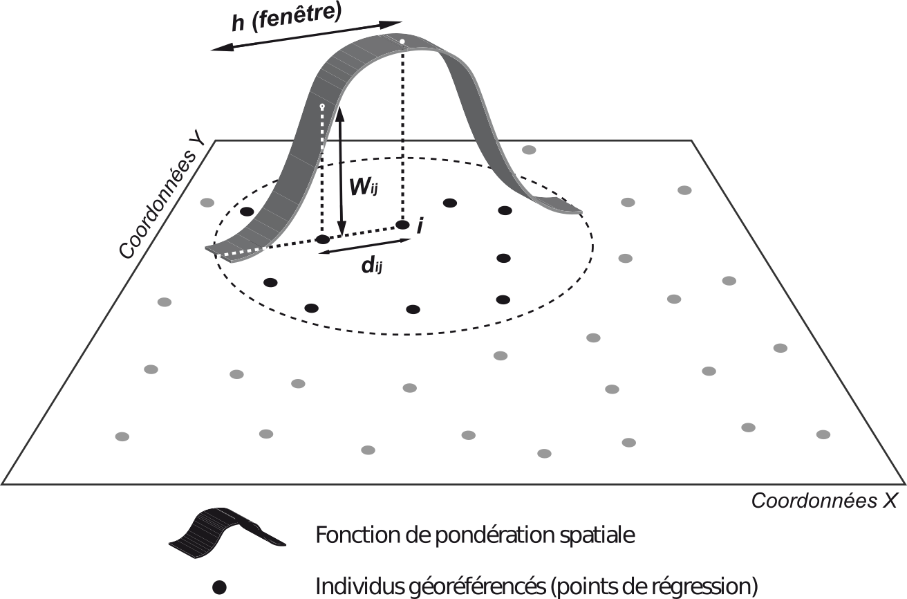
Source : Feuillet et al. (2019)
6.2 Calibration du modèle : définition et pondération du voisinage
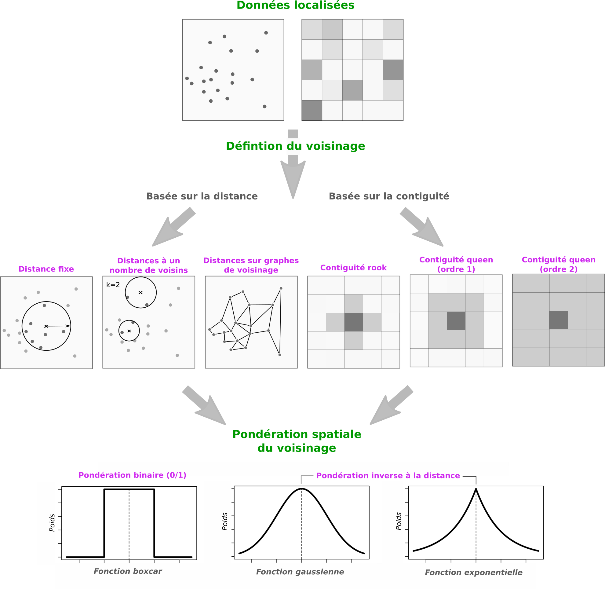
Source : Feuillet et al. (2019)
- Première chose à faire : convertir l’objet sf en objet sp
dataSp <- as_Spatial(dataSf) # le package GWmodel n'est pas compatible avec 'sf'6.2.1 Construction de la matrice de distances
matDist <- gw.dist(dp.locat = coordinates(dataSp))6.2.2 Optimisation du voisinage (h)
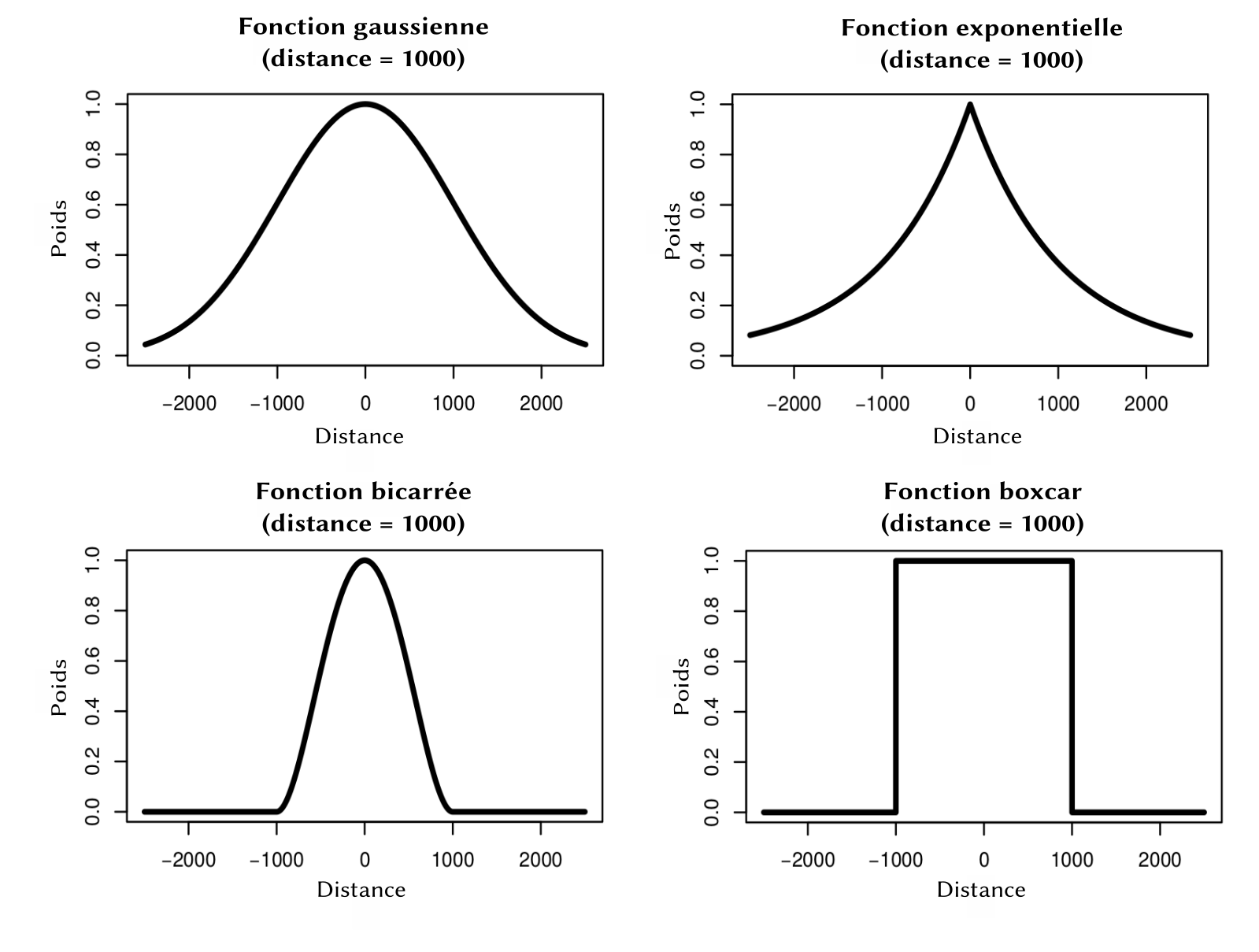
Source : Feuillet et al. (2019)
- Comparaison de deux pondérations spatiales : exponentielle et bicarrée :
# Exponential
nNeigh.exp <- bw.gwr(data = dataSp, approach = "AICc",
kernel = "exponential",
adaptive = TRUE,
dMat = matDist,
formula = log_valeur_fonciere ~ log_dist_litt + log_surface_reelle_bati + log_surface_terrain)Adaptive bandwidth (number of nearest neighbours): 280 AICc value: 413.5651
Adaptive bandwidth (number of nearest neighbours): 181 AICc value: 411.2085
Adaptive bandwidth (number of nearest neighbours): 118 AICc value: 409.2994
Adaptive bandwidth (number of nearest neighbours): 81 AICc value: 406.3428
Adaptive bandwidth (number of nearest neighbours): 56 AICc value: 404.8269
Adaptive bandwidth (number of nearest neighbours): 42 AICc value: 401.8334
Adaptive bandwidth (number of nearest neighbours): 32 AICc value: 398.9798
Adaptive bandwidth (number of nearest neighbours): 27 AICc value: 393.9232
Adaptive bandwidth (number of nearest neighbours): 23 AICc value: 394.5678
Adaptive bandwidth (number of nearest neighbours): 29 AICc value: 394.7075
Adaptive bandwidth (number of nearest neighbours): 25 AICc value: 394.9863
Adaptive bandwidth (number of nearest neighbours): 27 AICc value: 393.9232 # Bisquare
nNeigh.bisq <- bw.gwr(data = dataSp, approach = "AICc",
kernel = "bisquare",
adaptive = TRUE,
dMat = matDist,
formula = log_valeur_fonciere ~ log_dist_litt + log_surface_reelle_bati + log_surface_terrain)Adaptive bandwidth (number of nearest neighbours): 280 AICc value: 415.1779
Adaptive bandwidth (number of nearest neighbours): 181 AICc value: 414.4262
Adaptive bandwidth (number of nearest neighbours): 118 AICc value: 411.7238
Adaptive bandwidth (number of nearest neighbours): 81 AICc value: 417.0812
Adaptive bandwidth (number of nearest neighbours): 143 AICc value: 410.992
Adaptive bandwidth (number of nearest neighbours): 156 AICc value: 412.5089
Adaptive bandwidth (number of nearest neighbours): 132 AICc value: 410.2652
Adaptive bandwidth (number of nearest neighbours): 128 AICc value: 410.4043
Adaptive bandwidth (number of nearest neighbours): 137 AICc value: 410.9585
Adaptive bandwidth (number of nearest neighbours): 131 AICc value: 410.2002
Adaptive bandwidth (number of nearest neighbours): 128 AICc value: 410.4043
Adaptive bandwidth (number of nearest neighbours): 130 AICc value: 410.2136
Adaptive bandwidth (number of nearest neighbours): 128 AICc value: 410.4043
Adaptive bandwidth (number of nearest neighbours): 129 AICc value: 410.1641
Adaptive bandwidth (number of nearest neighbours): 132 AICc value: 410.2652
Adaptive bandwidth (number of nearest neighbours): 131 AICc value: 410.2002
Adaptive bandwidth (number of nearest neighbours): 131 AICc value: 410.2002
Adaptive bandwidth (number of nearest neighbours): 130 AICc value: 410.2136
Adaptive bandwidth (number of nearest neighbours): 130 AICc value: 410.2136
Adaptive bandwidth (number of nearest neighbours): 129 AICc value: 410.1641 6.3 Estimation de la GWR
# Avec pondération exponential
GWR.exp <- gwr.basic(data = dataSp, bw = nNeigh.exp, kernel = "exponential", adaptive = TRUE, dMat = matDist, formula = log_valeur_fonciere ~ log_dist_litt + log_surface_reelle_bati + log_surface_terrain)
# Avec pondération bisquare
GWR.bisq <- gwr.basic(data = dataSp, bw = nNeigh.bisq, kernel = "bisquare",
adaptive = TRUE, dMat = matDist,
formula = log_valeur_fonciere ~ log_dist_litt + log_surface_reelle_bati + log_surface_terrain)- Comparaison des deux calibrations :
diagGwr <- cbind(
rbind(nNeigh.exp,nNeigh.bisq),
rbind(GWR.exp$GW.diagnostic$gw.R2,GWR.bisq$GW.diagnostic$gw.R2),
rbind(GWR.exp$GW.diagnostic$AIC,GWR.bisq$GW.diagnostic$AIC)) %>%
`colnames<-`(c("Nb Voisins","R2","AIC")) %>%
`rownames<-`(c("EXPONENTIAL","BISQUARE"))
diagGwr Nb Voisins R2 AIC
EXPONENTIAL 27 0.6082865 340.0876
BISQUARE 129 0.5678470 372.1653- La GWR avec pondération exponentielle est la plus performante
- Interprétation des résultats bruts de la GWR :
GWR.exp ***********************************************************************
* Package GWmodel *
***********************************************************************
Program starts at: 2025-12-12 11:43:43.790761
Call:
gwr.basic(formula = log_valeur_fonciere ~ log_dist_litt + log_surface_reelle_bati +
log_surface_terrain, data = dataSp, bw = nNeigh.exp, kernel = "exponential",
adaptive = TRUE, dMat = matDist)
Dependent (y) variable: log_valeur_fonciere
Independent variables: log_dist_litt log_surface_reelle_bati log_surface_terrain
Number of data points: 442
***********************************************************************
* Results of Global Regression *
***********************************************************************
Call:
lm(formula = formula, data = data)
Residuals:
Min 1Q Median 3Q Max
-1.91270 -0.20171 0.02402 0.21625 1.33972
Coefficients:
Estimate Std. Error t value Pr(>|t|)
(Intercept) 9.97624 0.21722 45.927 < 2e-16 ***
log_dist_litt -0.08360 0.01926 -4.340 1.77e-05 ***
log_surface_reelle_bati 0.34515 0.04169 8.279 1.51e-15 ***
log_surface_terrain 0.25422 0.01823 13.942 < 2e-16 ***
---Significance stars
Signif. codes: 0 '***' 0.001 '**' 0.01 '*' 0.05 '.' 0.1 ' ' 1
Residual standard error: 0.3872 on 438 degrees of freedom
Multiple R-squared: 0.4934
Adjusted R-squared: 0.4899
F-statistic: 142.2 on 3 and 438 DF, p-value: < 2.2e-16
***Extra Diagnostic information
Residual sum of squares: 65.66596
Sigma(hat): 0.386317
AIC: 421.5673
AICc: 421.7049
BIC: 30.48042
***********************************************************************
* Results of Geographically Weighted Regression *
***********************************************************************
*********************Model calibration information*********************
Kernel function: exponential
Adaptive bandwidth: 27 (number of nearest neighbours)
Regression points: the same locations as observations are used.
Distance metric: A distance matrix is specified for this model calibration.
****************Summary of GWR coefficient estimates:******************
Min. 1st Qu. Median 3rd Qu. Max.
Intercept 7.875622 9.663876 10.063743 10.220684 10.8297
log_dist_litt -0.209386 -0.143417 -0.065722 -0.036018 0.2240
log_surface_reelle_bati -0.078886 0.255357 0.349362 0.413194 0.6410
log_surface_terrain 0.162807 0.227515 0.251227 0.269914 0.3646
************************Diagnostic information*************************
Number of data points: 442
Effective number of parameters (2trace(S) - trace(S'S)): 63.24453
Effective degrees of freedom (n-2trace(S) + trace(S'S)): 378.7555
AICc (GWR book, Fotheringham, et al. 2002, p. 61, eq 2.33): 393.9232
AIC (GWR book, Fotheringham, et al. 2002,GWR p. 96, eq. 4.22): 340.0876
BIC (GWR book, Fotheringham, et al. 2002,GWR p. 61, eq. 2.34): 113.0645
Residual sum of squares: 50.77133
R-square value: 0.6082865
Adjusted R-square value: 0.5427051
***********************************************************************
Program stops at: 2025-12-12 11:43:43.848609 - Première information : le R2 du modèle GWR est > au R2 du modèle MCO (plus grande capacité à expliquer la variance de Y).
- Seconde information : il semble exister une non-stationnarité spatiale, et même des inversions de signes pour la variable distance au littoral
Il faut maintenant cartographier les betas de chaque variable pour décrire cette non-stationnarité spatiale.
# Fonction de cartographie automatique des coefficients GWR
mapGWR <- function(spdf, var, var_TV, legend.title = "betas GWR", main.title) {
if (!inherits(spdf, "sf")) {
spdf <- st_as_sf(spdf)
}
tv <- spdf[abs(var_TV) > 1.96, ]
tm_shape(spdf) +
tm_dots(fill = var,
size = 0.5,
fill.legend = tm_legend(title = legend.title),
fill.scale = tm_scale_intervals(
style = "quantile",
n = 6,
values = "-RdYlBu",
midpoint = 0)) +
tm_shape(oleron) +
tm_lines(col = "black") +
tm_shape(tv) +
tm_dots(fill = "grey40", size = 0.1) +
tm_layout(title = main.title,
legend.title.size = 0.9,
inner.margins = 0.15)
}# Planche cartographique des 3 variables
a <- mapGWR(GWR.exp$SDF,
var = "log_dist_litt",
var_TV = GWR.exp$SDF$log_dist_litt_TV,
main.title = "Distance au littoral")
b <- mapGWR(GWR.exp$SDF,
var = "log_surface_reelle_bati",
var_TV = GWR.exp$SDF$log_surface_reelle_bati_TV,
main.title = "Surface bâtie")
c <- mapGWR(GWR.exp$SDF,
var = "log_surface_terrain",
var_TV = GWR.exp$SDF$log_surface_terrain_TV,
main.title = "Surface terrain")
tmap_arrange(a, b, c, ncol = 2)Bibliographie
Assunção, R. M., Neves, M. C., Câmara, G., & da Costa Freitas, C. (2006). Efficient regionalization techniques for socio‐economic geographical units using minimum spanning trees. International Journal of Geographical Information Science, 20(7), 797-811.
Feuillet, T., Commenges, H., Menai, M., Salze, P., Perchoux, C., Reuillon, R., … & Oppert, J. M. (2018). A massive geographically weighted regression model of walking-environment relationships. Journal of transport geography, 68, 118-129.
Feuillet, T., Cossart, E., & Commenges, H. (2019). Manuel de géographie quantitative: concepts, outils, méthodes. Armand Colin.
Fotheringham, A. S., Brunsdon, C., & Charlton, M. (2003). Geographically weighted regression: the analysis of spatially varying relationships. John Wiley & Sons.
Fotheringham, A. S., Yang, W., & Kang, W. (2017). Multiscale geographically weighted regression (MGWR). Annals of the American Association of Geographers, 107(6), 1247-1265.
Goodman, A. C., & Thibodeau, T. G. (1998). Housing market segmentation. Journal of housing economics, 7(2), 121-143.
Helbich, M., Brunauer, W., Hagenauer, J., & Leitner, M. (2013). Data-driven regionalization of housing markets. Annals of the Association of American Geographers, 103(4), 871-889.